Accurate summation
Accurate summation of two or more addends in floating-point arithmetic is not a trivial task. It has become an active field of research since the introduction of computers using floating-point arithmetic and resulted in many different approaches, that should only be sketched in Chapter Previous work. The accurate computation of sums is not only the basis for the chapter about accurate inner products, it is also important for residual iterations, geometrical predicates, computer algebra, linear programming or multiple precision arithmetic in general, as it is motivated in [Rump2009].
Previous work
Presorting the addends
One of the easiest summation algorithms is the Recursive summation (Algorithm
Recursive summation). Higham describes in [Higham2002] (Chapter 4)
that for this simple algorithm the order of the addends has a huge impact on the
accuracy of the resulting sum. The problem with presorting the data is, that
even fast sorting algorithms have a complexity of  and in many applications there is no information about the addends in advance
available. But the analyzing techniques and results from [Higham2002] (Chapter
4) can be applied later for other algorithms. Additional tools for error
analysis are given in [Brisebarre2010] (Chapter 6.1.2). For the purpose of
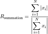
error analysis Higham introduces a condition number
and in many applications there is no information about the addends in advance
available. But the analyzing techniques and results from [Higham2002] (Chapter
4) can be applied later for other algorithms. Additional tools for error
analysis are given in [Brisebarre2010] (Chapter 6.1.2). For the purpose of
error analysis Higham introduces a condition number  for the addends:
(1)
1 2 3 4 5 6 | function [s] = RecursiveSummation(x, N) s = x(1); for i = 2:N s = s + x(i); end end |
If all addends have the same sign, then  . In
this case an increasing ordering is suggested. When the numbers of largest
magnitude are summed up first, all smaller addends will not influence the final
result, even if all small addends together would have a sufficient large
magnitude to contribute to the final result as well. If the signs of the largest
addends differ, then
. In
this case an increasing ordering is suggested. When the numbers of largest
magnitude are summed up first, all smaller addends will not influence the final
result, even if all small addends together would have a sufficient large
magnitude to contribute to the final result as well. If the signs of the largest
addends differ, then  and heavy
cancellation happens by computing
and heavy
cancellation happens by computing  . Such kind of
summation data is called ill-conditioned analogue to [Higham2002] (Chapter 4)
and has often the exact result zero. For this kind of addends Higham suggest a
decreasing pre ordering.
. Such kind of
summation data is called ill-conditioned analogue to [Higham2002] (Chapter 4)
and has often the exact result zero. For this kind of addends Higham suggest a
decreasing pre ordering.
Error-free transformation and distillation
The most basic error-free summation algorithms transform two input addends, e.g. a and b, into a floating-point sum x and a floating-point approximation error y. These algorithms are called error-free transformations [Ogita2005], if the following is satisfied:

It is easy to see, that if  is given,
  is valid too. The two most distinct instances fulfilling the
error-free transformation property are FastTwoSum (Algorithm
Error-free transformation FastTwoSum) by Dekker [Ogita2005] and TwoSum (Algorithm
Error-free transformation TwoSum) by Knuth [Ogita2005]. FastTwoSum requires three and
TwoSum six FLOP s. FastTwoSum additionally requires
is valid too. The two most distinct instances fulfilling the
error-free transformation property are FastTwoSum (Algorithm
Error-free transformation FastTwoSum) by Dekker [Ogita2005] and TwoSum (Algorithm
Error-free transformation TwoSum) by Knuth [Ogita2005]. FastTwoSum requires three and
TwoSum six FLOP s. FastTwoSum additionally requires  and thus unavoidably an expensive branch. So one has
to check for the individual use case whether three additional FLOP s
exceed the cost of a branch, see [Ogita2005] and [Brisebarre2010] (Chapter
4.3) . There exists another algorithm by Priest, which will not be taken into
account. It requires
and thus unavoidably an expensive branch. So one has
to check for the individual use case whether three additional FLOP s
exceed the cost of a branch, see [Ogita2005] and [Brisebarre2010] (Chapter
4.3) . There exists another algorithm by Priest, which will not be taken into
account. It requires  , thus a branch, and
more FLOP s than the two already presented algorithms [Brisebarre2010]
(Chapter 4.3.3).
, thus a branch, and
more FLOP s than the two already presented algorithms [Brisebarre2010]
(Chapter 4.3.3).
1 2 3 4 | function [x, y] = FastTwoSum (a, b) x = fl(a + b); y = fl(fl(a - x) + b); end |
1 2 3 4 5 | function [x, y] = TwoSum (a, b) x = fl(a + b); z = fl(x - a); y = fl(fl(a - fl(x - z)) + fl(b - z)); end |
The extension of error-free transformations from 2 to N addends is called distillation [Ogita2005].
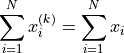
Distillation means, that in each distillation step k the values of the N
individual addends may change, but not their sum. The goal of distillation
algorithms is, that after a finite number of steps, assume k steps,
 approximates
  [Higham2002] (Chapter 4.4). The Error-free transformation and distillation
properties are preliminaries for cascaded and compensated summation.
[Higham2002] (Chapter 4.4). The Error-free transformation and distillation
properties are preliminaries for cascaded and compensated summation.
Cascaded and compensated summation
If FastTwoSum (Algorithm Error-free transformation FastTwoSum) or TwoSum (Algorithm
Error-free transformation TwoSum) is successively applied to all elements of a vector of
addends, it is called cascaded summation. When each new addend gets corrected
by the previously computed error of FastTwoSum (like in line 5 Algorithm
Kahan’s cascaded and compensated summation), it is called compensated
summation. The notation with explicit usage of FastTwoSum has been introduced
in [Brisebarre2010] (Algorithm 6.7). Algorithm Kahan’s cascaded and compensated summation relies on sorted input data  , because of the internal usage of FastTwoSum.
1 2 3 4 5 6 7 8 9 10 11 | % x: array of sorted addends % N: number of addends in x % s: computed sum function [s] = KahansCompensatedSummation (x, N) s = x(1); e = 0; for i = 2:N y = fl(x(i) + e); % compensation step [s, e] = FastTwoSum (s, y); end end |
Rump, Ogita and Oishi present in [Ogita2005] another interesting algorithm, namely SumK, which repeats the distillation k - 1 times, followed by a final recursive summation. The authors have shown that after the (k - 1)-th repetition of the cascaded summation, the result has improved, as if it has been computed with k-fold working precision.
Long and cascaded accumulators
A completely different approach is not to look for ways to cope with the errors of floating-point arithmetic, instead to change the precision on hardware level. Therefore Kulisch and Miranker proposed the usage of a long high-precision accumulator on hardware level [Kulisch1986]. This approach has not been realized so far by common hardware vendors. In his book Kulisch describes comprehensibly the realization of Scalar product computation units (SPU) for common 32 and 64 bit PC architectures or as coprocessors [Kulisch2013] (Chapter 8). Kulisch reports about two more or less successful attempts of coprocessor realizations, the most recent one with a Field Programmable Gate Array (FPGA) [Kulisch2013] (Chapter 8.9.3). The major issue is the time penalty of the much slower FPGA clock rates. But as there is much improvement on that field of research and with intelligent usage of parallelism, it might be possible to create a SPU, that is comparable to nowadays CPU floating-point units. Nevertheless the idea of the long accumulator resulted in a C++ toolbox called C-XSC [1], that is currently maintained by the University of Wuppertal. The C-XSC toolbox has been developed for several years and is thoroughly tested, therefore its version 2.5.3 will be used as reference for checking the correctness of the computed results later in Chapter Benchmark.
Another interesting approach came up in a paper by Malcom [Malcolm1971], who caught up Wolfes idea of cascaded accumulators. Malcom modified this idea by splitting each addend in order to add each split part to an appropriate accumulator. Finally all accumulators are summed up in decreasing order of magnitude using ordinary recursive summation. This case was treated in Chapter Presorting the addends and results in a small relative error [Higham2002] (Chapter 4.4).
Hybrid techniques
Zhu and Hayes published the accurate summation algorithm OnlineExactSum [Hayes2010]. This algorithm claims to be independent of the number of addends and the condition number (see Equation (1)) of the input. Furthermore the results of OnlineExactSum are correctly rounded. OnlineExactSum has a constant memory footprint, as it uses a fixed number of cascaded accumulators. Each addends exponent is examined for the choice of an appropriate accumulator and the accumulation is done by Dekkers error-free transformation algorithm FastTwoSum. In contrast to Malcoms approach, the final sum up of the cascaded accumulators is done by iFastSum [Hayes2009], a distillation algorithm like SumK. In their paper [Hayes2010] Zhu and Hayes proof the correctness of their algorithm by showing, that no accumulator looses any significant digits, and by the correctly rounded result of iFastSum for the final sum up. With various run time test for several types of input data they verified the stable and predictable behavior of OnlineExactSum. With this survey on previous work, a new algorithm will be proposed in the following chapter. Many ideas for the proposed algorithm accrued from this previous work and are extended by this new approach.
BucketSum
Generic description
The proposed algorithm BucketSum performs basically two steps, which will be explained comprehensively in this chapter:
- Sort and accumulate: N addends are sorted by magnitude and stored into
M buckets,
 . All significant bits are preserved.
 - Summing up buckets: compute an accurate sum of the M buckets.
This approach is already known from Zhu and Hayes algorithm HybridSum [Hayes2009] and from Malcolm [Malcolm1971]. Instead of increasing the precision of the accumulators, the input data is split and stored in several shorter accumulators. So each binary64 number can be seen as an extended-precision accumulator for the reduced input data precision. Like in HybridSum [Hayes2009] an array of binary64 numbers is created, each for accumulating a certain part of the full binary64 exponent range. Each element of that array will be called “bucket” in this chapter. For getting an overall picture, the algorithms for the steps 1 and 2 are presented first. The algorithm for step 2 is a slight modification of Kahan’s cascaded and compensated summation (Algorithm Kahan’s cascaded and compensated summation). The compensation step has been taken out of the for-loop to reduce the data dependency. In this modified version (Algorithm Modified Kahan’s cascaded and compensated summation) all summation errors are accumulated inside the for-loop for the final compensation step. Additionally an initial value for the resulting sum has been introduced.
1 2 3 4 5 6 7 8 | function [s] = ModifiedKahanSum (s, x, N) err = 0; for i = 1:N [s, e] = FastTwoSum (s, x(i)); err = fl(err + e); end s = fl(s + err) % compensation step end |
1 2 3 4 5 6 7 8 9 10 11 12 13 14 15 16 17 18 19 20 21 22 23 24 25 26 27 28 29 30 31 32 33 | function [s] = BucketSum (x, N) % Create appropriate masks mask = CreateMasks (M); mask(1) = 0; mask(M) = NaN; % Create array of M buckets, initialized with their mask. % a(1:2) are underflow and a((M - 1):M) are overflow buckets % a(3:(M - 2)) cover SHIFT exponents a = mask; sum = 0; for i = 1:N pos = ceil (exp(x(i)) / SHIFT) + 2; % exp(): extracts biased exponent [a(pos), e] = FastTwoSum (a(pos), x(i)); a(pos - 2) = fl(a(pos - 2) + e); if (mod (i, C1) == 0) % C1: capacity of normal buckets for j = 1:(M - 2) % Tidy up normal buckets r = fl(fl(mask(j + 1) + fl(a(j) - mask(j))) - mask(j + 1)); a(j + 1) = fl(a(j + 1) + r); a(j) = fl(a(j) - r); end end if (mod (i, C2) == 0) % C2: capacity of overflow buckets sum = fl(sum + fl(a(M - 1) - mask(M - 1))); % Tidy up overflow a(M - 1) = mask(M - 1); end end for i = 1:(M - 1) % Remove masks a(i) = a(i) - mask(i); end s = ModifiedKahanSum (sum, a_{M-1 \text{ downto } 1}, M-1); end |
BucketSum is responsible for step 1 and presented in Algorithm
BucketSum. What distinguishes BucketSum from OnlineExactSum is
the ternary partitioning of each floating-point accumulator (bucket). This
partitioning is done in order to archive a certain cascaded, overlapping pattern
for the accurate summation, as Figure Error storage scenario of the smallest allowed addend into bucket i - 2. shows. The
“distance” between two neighboring buckets is called shift and identical to
the length  in the partitioning. From Figure Generic significant partition. one can see, that the whole generic partitioning pattern
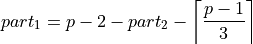
consists of the following parts, that are determined in Theorem 2:
in the partitioning. From Figure Generic significant partition. one can see, that the whole generic partitioning pattern
consists of the following parts, that are determined in Theorem 2:
- Two set bits in the beginning.
- Accumulation reserve (
 ): This length decides about the
number of addends, that can be accumulated into a bucket, without loosing
any significant bits.
): This length decides about the
number of addends, that can be accumulated into a bucket, without loosing
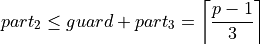
any significant bits. - Variable extension (guard): guard is a variable extension of the
following .
- Accumulated exponent range (): Each bucket is assigned to
accumulate addends of a certain exponent sub range. is the
length of this range. Therefore, is at least one, otherwise
no addend may be added to this bucket.
- Residual (
 ): is only used to preserve
significant bits of an addend.
): is only used to preserve
significant bits of an addend.
Another characteristic of BucketSum is, that there is no fixed splitting of the input addends like in HybridSum [Hayes2009]. The splitting is performed dynamically by FastTwoSum as one can see in Algorithm BucketSum line 9. After giving an overview of BucketSum, there follows a more detailed description of the algorithm, which starts with a formal analysis of the bucket partitioning.

Generic significant partition.
- Axiom 1.
- The “unit in the first place” (see Section Rounding) of a bucket is immutable except for the underflow or overflow range.
Axiom 1 means that during the summation process the significance of the most
significant bit of each bucket may not change. Otherwise it is not possible to
rely on a fixed exponent range for each bucket. To archive that, the leading bit
pattern “11” has been introduced. Under the assumption, that the most
significant bit of bucket i is  , each number less than
 may be added or subtracted without changing the significance
of the first bit of the bucket. This property is well known from integer
arithmetic.
may be added or subtracted without changing the significance
of the first bit of the bucket. This property is well known from integer
arithmetic.
- Assumption 1.
- The exponent range of floating-point numbers is unlimited.
Assumption 1 allows to ignore the under- and overflow-range for now. These two ranges will be treated in Section Realization for binary64 for the special case of binary64 values.
- Theorem 1.
- The summation error of bucket i has to be added at least to bucket i - 2.
- Proof.
- The proof for Theorem 1 will be done graphically in Figure
Four possible examples for partitioning and storing the error of the smallest
allowed addend into the neighbouring bucket.. In that Figure it is obvious, that
independent of the bit lengths , , and
the full bit precision p of the addend cannot be
preserved. Therefore the summation error of bucket i has to be added at
least to bucket i - 2, like shown in Figure
Error storage scenario of the smallest allowed addend into bucket i - 2.. In Algorithm BucketSum, line 10,
this action is performed. ∎

Four possible examples for partitioning and storing the error of the smallest allowed addend into the neighbouring bucket.

Error storage scenario of the smallest allowed addend into bucket i - 2.
- Assumption 2.
- The summation error of bucket i is added to bucket i - 2.
The choice of the error bucket is dependent on the size shift. The “further away” the error bucket is, the smaller shift has to be, as one might deduce from Figure Error storage scenario of the smallest allowed addend into bucket i - 2.. And the smaller shift is, the more buckets are required. Assumption 2 takes the first possible error bucket according to Theorem 1, in order to reduce the number of required buckets.
- Theorem 2.
For Axiom 1 , Assumption 1, and Assumption 2, the following rules have to apply to the lengths
, , and
 , in order to get a ternary bucket partition, that
maximizes the lengths and :
, in order to get a ternary bucket partition, that
maximizes the lengths and :- Proof.
From Figure Error storage scenario of the smallest allowed addend into bucket i - 2. three useful equations can be derived:
(2)

(3)

(4)

By reformulating Equation (2) to
 , one can derive
two equivalent objective functions
, one can derive
two equivalent objective functions  . For the latter one, a
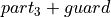
constrained optimization problem is given in (5).
. For the latter one, a
constrained optimization problem is given in (5).(5)
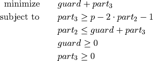
The optimization problem (5) can be relaxed to the problem (6) with additionally combining the first two constraints.
(6)
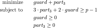
As
has the larger factor in the first constraint of
(6), an optimum can be
obtained for  in Equation (7).
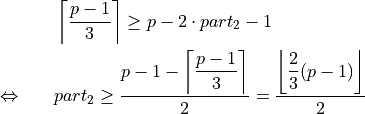
(7)
By respecting guard and
to be integers, an upward rounding
of this optimum, to fulfill the optimization constraints, yields the first
equation of Theorem 2. With the first equation of
Theorem 2 and equation (4)
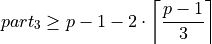
an upper bound for is found:(8)
A lower bound is obtained by combining
 and equation (3):
(9)
Respecting the integer property of
and by combining the
Equations (8) and (9), the
second equation of Theorem 2 is derived. Inserting the first equation
of Theorem 2 into Equation (2)
yields the third equation of Theorem 2. ∎
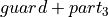
- Assumption 3.
- In the first equation of Theorem 2, guard is maximized.
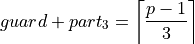
With Theorem 2 only an equation for the sum of guard and
was derived. As earlier described, guard is an extension , at
the cost of , which is of minor importance. Therefore it is more
desirable to maximize guard (Assumption 3). This allows to define guard
more precisely in Theorem 3.
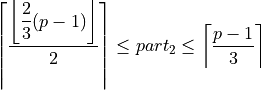
- Theorem 3.
- Under the Assumption 3 and with Theorem 2 it holds
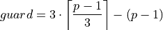 .
. - Proof.
According to Theorem 2
 is constant. This means
maximizing guard is equivalent to minimizing . A lower
bound for is given in Equation (3).
Combined with the upper bound of shift from the second equation of
Theorem 2, yields:
is constant. This means
maximizing guard is equivalent to minimizing . A lower
bound for is given in Equation (3).
Combined with the upper bound of shift from the second equation of
Theorem 2, yields:(10)
Due to the minimization of
, (10)
becomes an equation. This inserted into the first equation of Theorem 2,
proofs Theorem 3. ∎
All possible relations between shift and p can be seen in Figure All possible ternary partitions for a given shift. Note that p = 3 \cdot shift - 2 violates the upper bound of shift in Theorem 2.. In the following, the number of addends, that can be accumulated without loosing any significant bits, are described by Theorem 4.
All possible ternary partitions for a given shift. Note that  violates the upper bound of shift in Theorem 2.
- Theorem 4.
- Given the bucket partition of Theorem 2, up to
 additions to a bucket can be performed without violating Axiom 1.
 - Proof.
- Without loss of generality, the by magnitude largest allowed number to be
added to a bucket with a “unit in the first place” is
 .
The bucket is initialized with
.
The bucket is initialized with  , thus it will not
overflow for
, thus it will not
overflow for  . ∎
. ∎
Finally a complexity analysis of BucketSum (Algorithm BucketSum) similar to that one in [Hayes2010] should be done. For each of the N addends the following operations have to be performed:
- Bucket determination (line 8): 3 FLOP s [2]
- FastTwoSum (line 9): 3 FLOP s
- Error summation (line 10): 1 FLOP
After C2 steps, the overflow bucket has to be tidied up, that requires two
additional FLOP s (lines 18-21). After C1 steps, all M - 2 buckets
need to be tidied up. This requires five additional FLOP s (lines 11-17)
per bucket as well. Once in the end an unmasking has to happen with M - 1
FLOP s (lines 23-25) and for the final sum up, Algorithm
Modified Kahan’s cascaded and compensated summation (line 26) requires
 more FLOP s. All in all
![N \cdot 7 + \left\lfloor \dfrac{N}{C2} \right\rfloor \cdot 2 +
\left\lfloor \dfrac{N}{C1} \right\rfloor \cdot (M - 2) \cdot 5 +
\underbrace{(M - 1) + ((M - 1) \cdot 4) + 1}_{\text{Final sum up}} \quad
[FLOPs]](_images/math/1764e6ccd7cee97193f8039003c1a7360ff444d9.png)
are required. Assume a large number of addends . Then the final
sum up part has a small static contribution to the complexity, thus it can be
neglected. If the buckets don’t have to be tidied up during the summation for
small  , an overall complexity of 7N remains. Even if
 holds, the effort for tiding up is small compared to
the seven FLOP s, that always have to be performed. Thus the complexity
of BucketSum is considered to be 7N.
holds, the effort for tiding up is small compared to
the seven FLOP s, that always have to be performed. Thus the complexity
of BucketSum is considered to be 7N.
Realization for binary64
The binary64 type has the precision p = 53. Therefore we get
 and a significant
partitioning by Theorem 2 and Theorem 3, as shown in Figure
Significant partition for binary64..
and a significant
partitioning by Theorem 2 and Theorem 3, as shown in Figure
Significant partition for binary64..
Significant partition for binary64.
Also one can no longer assume an infinite exponent range. Assumption 1 has to
be replaced by a concrete bucket alignment. This alignment consists of three
parts, the under- and overflow and the normal bucket part. The anchor for the
alignment is, that the least significant bit of the shift part of the first
normal bucket a[0] has the significance of the biased exponent 0. This
anchor has been chosen, because no binary64, even the subnormal numbers
with a biased exponent of 0, can be accumulated into a bucket smaller than
a[0]. All in all to cover the full exponent range of binary64, one
needs  buckets. Beginning
with the first normal bucket a[0], each following bucket is aligned with a
unit in the first place of shift bigger than its predecessor. The maximal
multiple of shift that fits in this pattern is
buckets. Beginning
with the first normal bucket a[0], each following bucket is aligned with a
unit in the first place of shift bigger than its predecessor. The maximal
multiple of shift that fits in this pattern is  . Therefore we define the topmost bucket to be an
overflow bucket. This bucket is responsible for values with a unit in the first
place of greater than
. Therefore we define the topmost bucket to be an
overflow bucket. This bucket is responsible for values with a unit in the first
place of greater than  , but these values are ignored in this
work. With an unreasonable effort, this overflow situation can be handled
differently. The second overflow bucket needs an exceptional alignment as well.
Its is smaller due to upper limit of the binary64
exponent range
, but these values are ignored in this
work. With an unreasonable effort, this overflow situation can be handled
differently. The second overflow bucket needs an exceptional alignment as well.
Its is smaller due to upper limit of the binary64
exponent range  . Because of the alignment of a[0] and
Assumption 2, two additional error buckets for the underflow range are
required. For the underflow range
. Because of the alignment of a[0] and
Assumption 2, two additional error buckets for the underflow range are
required. For the underflow range ![[2^{-1023}, \; 2^{-1074}]](_images/math/0efd75a7daee1f3232baa34518bdf30e030099cd.png) , bucket
a[-1] follows the alignment scheme of the normal buckets and bucket a[-2] is
responsible for the remaining bit positions. The exponent range partition is
illustrated in Equation (11). Graphical
visualizations of the bucket alignment in the under- and overflow range are
given in the Figures Visualization of the bucket alignment in the underflow range. and
Visualization of the bucket alignment in the overflow range..
, bucket
a[-1] follows the alignment scheme of the normal buckets and bucket a[-2] is
responsible for the remaining bit positions. The exponent range partition is
illustrated in Equation (11). Graphical
visualizations of the bucket alignment in the under- and overflow range are
given in the Figures Visualization of the bucket alignment in the underflow range. and
Visualization of the bucket alignment in the overflow range..
(11)¶![\begin{aligned}
&\overbrace{\underbrace{2^{1010} \cdots 2^{993}}_{a[112]}}^{\text{overflow bucket}}
\underbrace{2^{992} \cdots 2^{975}}_{a[111]}
\underbrace{2^{974} \cdots 2^{957}}_{a[110]} \cdots \\
&\qquad\cdots \underbrace{2^{-1006} \cdots 2^{-1023}}_{a[0]}
\overbrace{\underbrace{2^{-1024} \cdots 2^{-1041}}_{a[-1]}
\underbrace{2^{-1042} \cdots 2^{-1074}}_{a[-2]}}^{\text{underflow buckets}}
\end{aligned}
Exponent range partition.](_images/math/20c69a6ff0eff4e65ff05a16b117e9a3e554a6b4.png)
Finally the accumulation reserve for the normal and underflow buckets is
according to Theorem 4 smaller than  . For the first overflow
bucket one obtains analogue to Theorem 4 an accumulation reserve of less than
. For the first overflow
bucket one obtains analogue to Theorem 4 an accumulation reserve of less than
 .
.
Implementation
One essential element of this project is the efficient implementation of BucketSum. This chapter deals with all implementation details and changes to the pseudo-code from Algorithm BucketSum. Some potential improvements to a floating-point using software are described in Chapters Software and compiler support and Performance. The in Chapter Performance presented technique of partial loop unrolling can be used to obtain an elegant side effect for the tidy up and sum up steps. In Algorithm BucketSum all buckets are initialized with an appropriate mask. This mask has to be considered in the tidy up process (lines 13 and 19-20) and it has to be removed before the final sum up (lines 23-25). If two different bucket arrays a1 and a2 are used, a1 uses the masks as described in Algorithm BucketSum and a2 uses the negative masks. In that way the exact sum of the unmasked values of the buckets i can be computed by a1[i] + a2[i]. This way the number of floating-point operations dealing with masking and unmaking are reduced a lot. Additionally the partial loop unrolling increases the instruction-level parallelism and finally increases the tidy up values by a factor of two. This means that less tidy up “interruptions” for the N addends are required.
Another considered optimization is the avoidance of the division by the shift in Algorithm BucketSum line 8. An integer division is an expensive operation compared to multiplication and bit shifting. In [Fog2014] (p. 54-58) one can find latencies for several instructions. For the AMD “Piledriver” the latency for a signed or unsigned division ((I)DIV [AMD2013b] (Chapter 3)) ranges from 12-71 clock cycles. Compared to this the sum of the latencies of a left or right bit shift (SHL/SHR [AMD2013b] (Chapter 3)) with one clock cycle and a signed or unsigned multiplication ((I)MUL [AMD2013b] (Chapter 3)) with 4-6 clock cycles is by far smaller. As this division by the shift has to be done for each addends exponent, a small speed up could be archived by replacing the division by a multiplication followed by a bit shift, as shown in Listing Division by 18 replacement. The idea behind the values of Listing Division by 18 replacement is an integer optimization problem.
(12)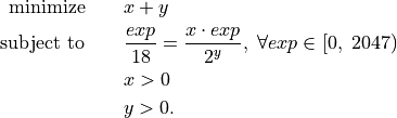
For normal and subnormal binary64 the exponents range from 0 to 2046 and
the desired division should be a cheap bit shift, thus a power of two.
Therefore the task is to find for the smallest possible power of two y some
minimal  . This x was
found with the program of Listing Program to solve the integer optimization problem (Equation eq-Division by 18 optimization problem)..
. This x was
found with the program of Listing Program to solve the integer optimization problem (Equation eq-Division by 18 optimization problem)..
1 2 3 4 5 6 | double d = 1.0; // Exponent extraction unsigned position = ((ieee754_double *)(&d))->exponent; // Perform equivalent operations unsigned pos1 = position / 18; unsigned pos2 = (position * 1821) >> 15; |
1 2 3 4 5 6 7 8 9 10 11 12 13 14 15 16 17 18 19 20 21 22 23 24 | #include <cmath> #include <iostream> int main () { unsigned div = 1; // Try some powers of two (div = 2^y) for (unsigned y = 1; y < 32; y++) { div *= 2; unsigned x = (unsigned) std::ceil ((double) div / 18.0); // Test all exponents of the IEEE 754 - 2008 binary64 normal and // subnormal range int is_valid = 1; for (unsigned i = 0; i < 2047; i++) { is_valid &= ((i / 18) == ((i * x) / div)); } if (is_valid) { std::cout << "Found: " << x << " / 2^" << y << std::endl; } } return 0; } |
Benchmark
The benchmark program compares the five summation algorithms of Table Comparison of summation algorithms for input data length N with their source of implementation mentioned in brackets. The accurate summation results of the C-XSC toolbox will be used as reference values for the five types of test data.
| Algorithm | FLOP s | Run-time | Space |
|---|---|---|---|
| Ordinary Recursive Summation (Algorithm Recursive summation) |  |
1 |  |
| SumK (K = 2, [Lathus2012]) |  |
2-3 |  |
| iFastSum ([Hayes2010]) |  |
3-5  |
|
| OnlineExactSum ([Hayes2010]) |  |
4-6*  |
|
| BucketSum (Algorithm BucketSum) |  |
1-2* | |
An asterisk “*” in Comparison of summation algorithms for input data length N indicates the
use of instruction-level parallelism, a dagger “”, that the
results for Data 3 were omitted, and a double dagger “”, that
this applies only for large dimensions. The test data for the summation
benchmark program is chosen similar to [Hayes2010]. Data 1 are N random,
positive floating-point numbers, all with an exponent of  . Thus
Data 1 is pretty well-conditioned . Data 2
is ill-conditioned. The exponents are distributed uniformly and randomly between
. Thus
Data 1 is pretty well-conditioned . Data 2
is ill-conditioned. The exponents are distributed uniformly and randomly between
 and
and  , the signs are assigned randomly and the
significant is filled randomly as well. Data 3 is similar to Data 2, but its
sum is exactly zero. Data 4 is Anderson’s ill-conditioned data
[Anderson1999]. And finally Data 5 is designed to especially stress the
accumulation reserve of BucketSum. A visualization of that test case is given
in Figure Visualization of the stress test case for roundToNearest..
, the signs are assigned randomly and the
significant is filled randomly as well. Data 3 is similar to Data 2, but its
sum is exactly zero. Data 4 is Anderson’s ill-conditioned data
[Anderson1999]. And finally Data 5 is designed to especially stress the
accumulation reserve of BucketSum. A visualization of that test case is given
in Figure Visualization of the stress test case for roundToNearest..
For time measurement the clock() function [ISO-IEC-9899-2011] (Chapter
7.27.2.1) [ISO-IEC-14882-2011] (Chapter 20.11.8) is used. To keep the time
measurement as accurate as possible, all memory operations like array creation
and destruction should be kept outside of time measuring code blocks. On the
other hand, if the size of the input data N was chosen too small, the measured
time is too inaccurate. This requires a certain number of repeated operations
R, to obtain detectable results. But some algorithms like SumK and
iFastSum operate inline on the input data. Thus providing a single copy of the
data will not suffice to get identical initial conditions for each repetition.
To meet all these constraints, a large copy of  elements
for summation is created, each of the repeated N elements with a leading zero,
as iFastSum and BucketSum imitate Fortran indexing. The systems available
main memory creates another constraint on the maximum test case size
elements
for summation is created, each of the repeated N elements with a leading zero,
as iFastSum and BucketSum imitate Fortran indexing. The systems available
main memory creates another constraint on the maximum test case size  . This product should not exceed the test systems 8 GB of main
memory, otherwise the timings will become inaccurate due to swapping to hard
disk. This means for R = 1 repetitions the theoretical maximum test case size
can be
. This product should not exceed the test systems 8 GB of main
memory, otherwise the timings will become inaccurate due to swapping to hard
disk. This means for R = 1 repetitions the theoretical maximum test case size
can be
Experimental test runs revealed, that about  elements are
necessary in order to obtain detectable results. Therefore the following data
lengths and repetitions are defined:
elements are
necessary in order to obtain detectable results. Therefore the following data
lengths and repetitions are defined:
- Middle dimension:
![\left[10^{3}, 10^{4}\right]](_images/math/9816a129e1f5f3ad010fdf5e709391e934ebbf7b.png) elements with
elements with
 repetitions
 - Large dimension:
![\left[10^{6}, 10^{7}\right]](_images/math/2d48950067fabdcc26715e6fb45e8c52b9487d65.png) elements with
elements with
 repetitions
Well-conditioned .
Ill-conditioned.
Ill-conditioned  .
.
Anderson’s ill-conditioned data.
Stress test.
Well-conditioned .
Ill-conditioned.
Ill-conditioned .
Anderson’s ill-conditioned data.
Stress test.
The benchmarks (see Figures above) show, that BucketSum performs best for all
given kinds of data. BucketSum is by factor 2-3 slower than the Ordinary
Recursive Summation and is slightly faster than SumK (with K = 2). For
middle and large data lengths BucketSum scales linear in contrast to
OnlineExactSum, which starts to scale linear at a data length of about
 elements. Another interesting observation is, that
OnlineExactSum is dependent on the condition of the input data
for small data lengths. For iFastSum,
OnlineExactSum and BucketSum the results have been compared to that one of
the C-XSC toolbox using an assert() [ISO-IEC-14882-2011] (Chapter 19.3)
statement, thus any inaccurate result would have interrupted the benchmark. As
no interruptions occurred, all three algorithms are assumed to deliver correctly
rounded sums. The most important properties of the algorithms under test are
summarized in Table Comparison of summation algorithms for input data length N, which is a
modified extension of [Hayes2010].
elements. Another interesting observation is, that
OnlineExactSum is dependent on the condition of the input data
for small data lengths. For iFastSum,
OnlineExactSum and BucketSum the results have been compared to that one of
the C-XSC toolbox using an assert() [ISO-IEC-14882-2011] (Chapter 19.3)
statement, thus any inaccurate result would have interrupted the benchmark. As
no interruptions occurred, all three algorithms are assumed to deliver correctly
rounded sums. The most important properties of the algorithms under test are
summarized in Table Comparison of summation algorithms for input data length N, which is a
modified extension of [Hayes2010].
Footnotes
| [1] | http://www2.math.uni-wuppertal.de/wrswt/xsc/cxsc_new.html |
| [2] | For simplicity integer operations are counted as FLOP s. |