Accurate inner product¶

With the FMA instruction and an efficient and fast summation algorithm, one is able to create efficient inner product algorithms as well. After a short overview about previous approaches, three algorithms using FMA will be introduced.

Previous work¶

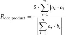
Like the recursive summation (Algorithm Recursive summation), there also exists a simple straight forward implementation of the inner product, namely Algorithm Recursive inner product, see [Brisebarre2010] (Algorithm 6.2). A condition number for the inner product (Equation (1)) is defined in [Brisebarre2010] (Chapter 6.1.2) as well:

(1)¶ $R_{\text{dot product}} = \dfrac{2 \cdot \displaystyle\sum_{i = 1}^{n} \vert a_{i} \cdot b_{i}\vert} {\left\vert\displaystyle\sum_{i = 1}^{n} a_{i}\cdot b_{i}\right\vert}$

Recursive inner product¶

function [s] = RecursiveDotProduct (a, b, N)
  s = fl(a(1) * b(1));
  for i = 2:N
    s = fl(s + fl(a(i) * b(i)));
  end
end

Similar to the definition of the error-free transformation for the sum, there also exists a definition for the product in [Ogita2005]:

(2)¶ $a \cdot b = x + y \quad\text{and}\quad x = fl(a \cdot b)$

This means the product is transformed into a sum. By knowing this, it becomes obvious why the task of finding an efficient inner product algorithm is strongly connected with the task of accurate summation. If the factors are floating-point numbers $a, b \in \mathbb{F}$ , then $x, y \in \mathbb{F}$ holds, like for the error-free transformation of the sum, too. $x \in \mathbb{F}$ follows from the definition in Equation (2). 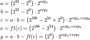An example for $y \in \mathbb{F}$ for the special case of binary64 is given in Equation (3). If a and b have the biggest possible significant (all bits set to “1”), then their product cannot exceed 106 bits. This fits exactly into two 53 bit precisions of a binary64.

(3)¶ $\begin{aligned} a &= \left(2^{53} - 2^{0}\right) \cdot 2^{exp_{a}} \nonumber \\ b &= \left(2^{53} - 2^{0}\right) \cdot 2^{exp_{b}} \nonumber \\ c &= a \cdot b = \left(2^{106} - 2^{54} + 2^{0}\right) \cdot 2^{exp_{a} + exp_{b}} \\ x &= fl(c) = \left(2^{106} - 2^{54}\right) \cdot 2^{exp_{a} + exp_{b}} \nonumber \\ y &= a \cdot b - fl(c) = \left(2^{0}\right) \cdot 2^{exp_{a} + exp_{b}} \nonumber \end{aligned}$

Without the FMA instruction, there exists the algorithm TwoProduct, that is able to perform this error-free product transformation by using 17 FLOP s, see [Ogita2005]. Having a system with a hardware implemented FMA instruction, the whole effort can be reduced to TwoProductFMA (Algorithm Error-free transformation TwoProductFMA). This algorithm is also described in [Ogita2005] and requires only two FLOP s.

Error-free transformation TwoProductFMA¶

function [x, y] = TwoProductFMA (a, b)
  x = fl(a * b);
  y = FMA(a, b, -x);
end

For the inner product the idea of error-free transformation can also be extended from two to N operands with Dot2 (Algorithm Inner product in twice the working precision Dot2). Dot2 computes $\sum_{i = 1}^{N} x_{i} \cdot y_{i}$ as if twice the working precision was used [Ogita2005]. In that paper the idea has been extended to algorithm DotK, which can evaluate the inner product, as if computed with K-fold working precision. A slightly modified version of Dot2 will be presented in the next chapter.

Inner product in twice the working precision Dot2¶

function [p] = Dot2 (x, y, N)
  [p, s] = TwoProduct (x(1), y(1));
  for i = 2:N
    [h, r] = TwoProduct (x(i), y(i));
    [p, q] = TwoSum (p, h);
    s = fl(s + fl(q + r));
  end
  p = fl(p + s);
end

Algorithms based upon TwoProductFMA¶

The first algorithm that is tested in the following benchmark (Chapter Benchmark) is Dot2 (Algorithm Inner product in twice the working precision Dot2) with all occurrences of TwoProduct replaced by TwoProductFMA. This algorithm will be called Dot2FMA in the following. This modification is already described in [Ogita2005].

Another trivial idea is not to modify the existing summation algorithms of Chapter Accurate summation. Instead a preprocessing of the input vectors is done with TwoProductFMA (Algorithm Error-free transformation TwoProductFMA). This approach will be called FMAWrapperDotProd and is described in Algorithm FMAWrapperDotProd transforms a dot product into sum and finally calls BucketSum. in combination with BucketSum. FMAWrapperDotProd has two major flaws. The first one is connected with the data preprocessing. The implementer has to decide whether the method should preserve the input vectors or not. In the first case the memory requirement increases by twice the size of the input vector length, in the latter case the original input vectors are lost. The second flaw is related to the usage of the summation algorithm in Algorithm FMAWrapperDotProd transforms a dot product into sum and finally calls BucketSum. lines 7-8. These lines create an intermediate rounding, that dependent on the resulting vectors can return a not correctly rounded result. A solution to this problem would be an interface method, that allows to accumulate a vector of a certain size, and a second one to make a final sum up to a correctly rounded sum. Such an interface is for example available in the implementation of OnlineExactSum [Hayes2010].

FMAWrapperDotProd transforms a dot product into sum and finally calls BucketSum.¶

function [s] = FMAWrapperDotProd(x, y, N)
  for i = 1:N                    % In-place array preprocessing
    t = fl(x(i) * y(i));         % Destructive TwoProductFMA
    y(i) = FMA(x(i), y(i), -t);
    x(i) = t;
  end
  s = BucketSum (x, N);          % Any summation algorithm possible
  s = fl(s + BucketSum (y, N));
end

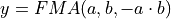Finally a modified version of BucketSum (Algorithm BucketSum) is presented, namely BucketDotProd (Algorithm BucketDotProd). BucketDotProd is identical to BucketSum, except for the lines 8-13, where TwoProductFMA comes into play. Assume the product to accumulate is $a \cdot b$ , therefore $x = fl(a \cdot b)$ and $y = FMA(a, b, -a \cdot b)$ . It was already shown, that if x has to be added to bucket i and its error to bucket i - 2, no significant bit is lost (Theorem 1). In order to avoid the expensive three FLOP s for the exponent extraction of y, one can make use of the shift = 18 property for the binary64 realization. In that case y will always fall in the exponent range of bucket i - 3. According to Theorem 1 the error of y has to be added to bucket i - 5.

Visualization of BucketDotProds accumulation.

BucketDotProd¶

function [s] = BucketDotProd (x, y, N)
  % Create appropriate masks
  mask = CreateMasks (M);
  mask(1) = 0;
  mask(M) = NaN;

  % Create array of M buckets, initialized with their mask.
  %   a(1:2) are underflow and a((M - 1):M) are overflow buckets
  %   a(3:(M - 2)) cover SHIFT exponents
  a = mask;

  sum = 0;
  for i = 1:N
    [v, w] = TwoProductFMA (x(i), y(i));
    pos = ceil (exp(v) / SHIFT) + 2;        % exp(): extracts biased exponent
    [a(pos), e(1)] = FastTwoSum (a(pos), v);
    [a(pos - 3}, e(2)) = FastTwoSum (a(pos - 3}, w);
    a(pos - 2) = fl(a(pos - 2) + e(1));
    a(pos - 5) = fl(a(pos - 5) + e(2));
    if(mod (i, C1) == 0)                     % C1: capacity of normal buckets
      for j = 1:(M - 2)                              % Tidy up normal buckets
        r = fl(fl(mask(j + 1) + fl(a(j) - mask(j))) - mask(j + 1));
        a(j + 1) = fl(a(j + 1) + r);
        a(j) = fl(a(j) - r);
      end
    end
    if (mod (i, C2) == 0)                  % C2: capacity of overflow buckets
      sum = fl(sum + fl(a(M - 1) - mask(M - 1)));          % Tidy up overflow
      a(M - 1) = mask(M - 1);
    end
  end
  for i = 1:(M - 1)        % remove masks
    a(i) = a(i) - mask(i);
  end
  s = ModifiedKahanSum (sum, a_{M-1 \text{ downto } 1}, M-1);
end

This chapter shows, that with moderate effort nearly each summation algorithm can be modified to handle the task of inner product computation as well. In the following numerical tests show the properties of these three algorithms in a benchmark program.

Benchmark¶

For the benchmark of inner product the five algorithms of Table Comparison of inner product algorithms for input data length N are compared. All algorithms were implemented as part of this work. Only for the implementation of Dot2 and Dot2FMA some sub-functions of [Lathus2012] were used. Like for the summation benchmark the C-XSC toolbox has been used to verify the correctness of the computed inner products.

Comparison of inner product algorithms for input data length N¶
Algorithm	FLOP s	Run-time	Space
Recursive Inner Product (Algorithm Recursive inner product)	$2N-1$	1	$\mathcal{O}(1)$
Dot2 (Algorithm Inner product in twice the working precision Dot2)	$25N-7$	5-6	$\mathcal{O}(1)$
Dot2FMA (Algorithm Inner product in twice the working precision Dot2)	$6N-3$	3-4	$\mathcal{O}(1)$
FMAWrapperDotProd (Algorithm FMAWrapperDotProd transforms a dot product into sum and finally calls BucketSum.)	$16N$	4-6*	$\mathcal{O}(N)$
BucketDotProd (Algorithm BucketDotProd)	$13N$	3-4*	$\mathcal{O}(1)$

The asterisk “*” in Comparison of inner product algorithms for input data length N indicates the use of instruction-level parallelism. For the inner product benchmark four kinds of test data are used. Data 1 are two random, positive floating-point vectors of length N, all with an exponent of $2^{0}$ . Data 2 is well-conditioned like Data 1, but each of the two input vectors has a random distributed exponent range between $2^{0}$ and $2^{400}$ . Data 3 is ill-conditioned with a random distributed exponent between $2^{-400}$ and $2^{400}$ . Finally Data 4 is ill-conditioned, with a real inner product of exactly zero. The time measuring and the determination of the middle and large dimension data lengths happens in the same way as in Chapter Benchmark. Especially the assumptions for the data length determination allows the creation of two arrays, without exceeding the available main memory.

Well-conditioned, equal exponent.

Well-conditioned, large exponent range.

Ill-conditioned, large exponent range.

Well-conditioned, equal exponent.

Well-conditioned, large exponent range.

Ill-conditioned, large exponent range.

Ill-conditioned, zero result.

The results of the inner product benchmark, shown in Figures above, verify a linear scaling of the algorithms in Table Comparison of inner product algorithms for input data length N for data lengths in each, middle and large dimension. Another observation is, that the type of the data does not really affect the runtime of the algorithms. In any case BucketDotProd is the fastest algorithm and only by factor 2-3 slower than the Recursive Inner Product. FMAWrapperDotProd, that only preprocesses the input vectors, is already by factor 4-6 slower than the Recursive Inner Product. The reason for this seems to be, that all input vectors have to be processed completely twice. Another improvement is observable if Dot2 is used in combination with TwoProductFMA in Dot2FMA. The execution time nearly halves, if a hardware implemented FMA instruction is available on the system. The result accuracy is again checked by an assert()-statement against the result of the C-XSC toolbox, like it was done for the summation benchmark. Therefore the results of BucketDotProd are claimed to be correctly rounded. This check cannot be applied for FMAWrapperDotProd, because of the in the previous chapter discussed implementation drawback.